
Getting started
imagefluency: Image Statistics Based on Processing Fluency
April 01, 2026
Source:vignettes/getting-started.Rmd
getting-started.RmdIntroduction
Motivation: Why create yet another R package
Over the last decades, the amount of data generated is growing rapidly, predominantly due to digitalization. Most of today’s data is unstructured, and this share is increasing. Given that unstructured data is rich, these data could provide rich insights for scientific research from a variety of fields and practice alike. Especially images (i.e., visual stimuli) are recognized as valuable source of information.
At the same time, vision research and research in psychology shows that even simple changes in low-level image features (like symmetry, contrast, or complexity) can have a tremendous effect on a variety of human judgments. As an example, a statement like “Nut bread is healthier than potato bread” is more likely to be perceived as true when presented in a color that is easy to read against a white background (high contrast) instead of being presented in a color that is difficult to read against a white background (low contrast; cf. [1]). Thus, it might be useful to estimate and control for differences in such low-level visual features in any research that includes visual stimuli.
imagefluency is an R package for such
low-level image scores based on processing fluency theory. The package
allows to get scores for several basic aesthetic principles that
facilitate fluent cognitive processing of images: contrast, complexity /
simplicity, self-similarity, symmetry, and typicality.
Why and when to use the package
Possible applications include:
- stimulus selection in experiments (e.g., testing brand logos, evaluate product designs, online display ads)
- as control variables in statistical or prediction models
- linking image fluency scores to outcomes of interest (e.g., how should a typical product packaging look like, do simpler images get more or less attention on a website, …)
- (interpretable) image features in simple machine learning models, e.g. SVM image classifier
Theoretical background
The most prevailing explanation for how low-level image features affect human judgments is based on processing fluency theory [2]. Processing fluency describes the ease of processing a stimulus [3], which happens instantaneously and automatically [4]. Higher processing fluency results in a gut-level positive affective response [5]. Notably, a rich body of literature has shown that processing fluency effects have an impact on a variety of judgmental domains in our everyday life, including how much we like things, how much we consider statements to be true, how trustworthy we judge a person, how risky we think something is, or whether we buy a product or not (for a review, see [6]).
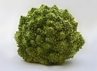
Several stimulus features have been proposed that result in increased fluency. In particular, visual symmetry, simplicity, (proto-)typicality, and contrast were identified to facilitate processing [2]. Recent studies further discuss self-similarity in light of fluency-based aesthetics [7, 8], a concept which has been studied for example in images of natural scenes [9]. Self-similarity can be described as self-repeating patterns within a stimulus. A typical example are the leaves of ferns that feature the same shape regardless of any magnification or reduction (i.e., scale invariance). Another prominent example is romanesco broccoli with its self-similar surface.
Extracting image features for contrast, self-similarity, simplicity,
symmetry, and typicality therefore constitute the core purpose of the
imagefluency package.
Package overview
Main functions
-
img_contrast()visual contrast of an image -
img_complexity()visual complexity of an image (opposite of simplicity) -
img_self_similarity()visual self-similarity of an image -
img_simplicity()visual simplicity of an image (opposite of complexity) -
img_symmetry()vertical and horizontal symmetry of an image -
img_typicality()visual typicality of a list of images relative to each other
Other helpful functions
-
img_read()reads bitmap images into R -
rgb2gray()converts images from RGB into grayscale (might speed up computation) -
run_imagefluency()to launch a Shiny app locally on your computer for an interactive demo of the main functions (alternatively, visit the online version at posit.cloud)
Installation
You can install the current stable version from CRAN.
install.packages('imagefluency')To download the latest development version from Github use the
install_github function of the remotes
package.
# install remotes if necessary
if (!require('remotes')) install.packages('remotes')
# install imagefluency from github
remotes::install_github('stm/imagefluency')
After installation, the imagefluency package is loaded
the usual way by calling library(imagefluency). The
img_read() function can be used to read an image into R.
Just like with reading in a dataset, img_read() expects the
path to the file as input, e.g.,
img_read('C:/Users/myname/Documents/myimage.jpg').
Currently supported file formats are bmp, jpg, png, and tif.
Use the following link to report bugs/issues: https://github.com/stm/imagefluency/issues
Using imagefluency
imagefluency allows to get scores for five image
features that facilitate fluent processing of images: contrast,
complexity / simplicity, self-similarity, symmetry, and typicality.
To use the imagefluency package, first load the library.
Contrast
The function img_contrast() returns the contrast of an
image. Most research defines contrast in images as the root-mean-squared
(RMS) contrast which is the standard deviation of the normalized pixel
intensity values [10]:
.
The RMS of an image as a measure for visual contrast has been shown to
predict human contrast detection thresholds well [11]. Therefore,
the function calculates contrast by computing the RMS contrast of the
input image. Consequently, a higher value indicates higher contrast. The
image is normalized if necessary (i.e., normalization into range [0,
1]). For color images, a weighted average between color the channels is
computed (cf. [8]).
Note that in the following, example images that come with the package
are used. Moreover, the images can be displayed using the
grid.raster() function from the grid
package.
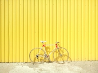
# Example image with relatively high contrast: berries
berries <- img_read(system.file('example_images', 'berries.jpg', package = 'imagefluency'))
# display image
grid::grid.raster(berries)
# get contrast
img_contrast(berries)
# Example image with relatively low contrast: bike
bike <- img_read(system.file('example_images', 'bike.jpg', package = 'imagefluency'))
# display image
grid::grid.raster(bike)
# get contrast
img_contrast(bike)
Calculating the contrast scores for the two images gives the following result:

Complexity / Simplicity
The function img_complexity() returns the visual
complexity of an image. Algorithmic information theory indicates that
picture complexity can be measured accurately by image compression rates
because complex images are denser and have fewer redundancies [12, 13]. Therefore, the function
calculates the visual complexity of an image as the ratio between the
compressed and uncompressed image file size. Thus, the value does not
depend on image size.
The function takes the file path of an image file (or URL) or a
pre-loaded image as input argument and returns the ratio of the
compressed divided by the uncompressed image file size. The complexity
values are naturally interpretable and can range between almost 0
(virtually completely compressed image, thus extremely simple image) and
1 (no compression possible, thus extremely complex image). The function
offers to use different image compression algorithms like
jpg, gif, or png with
algorithm = 'zip' as default (for a discussion about the
different algorithms, see [8]).
As most compression algorithms do not depict horizontal and vertical
redundancies equally, the function includes an optional
rotate parameter (default: FALSE). Setting
this parameter to TRUE additionally creates a compressed
version of the rotated image. The overall compressed image’s
file size is computed as the minimum of the original image’s file size
and the file size of the rotated image.
The function img_simplicity() returns the visual
simplicity of an image. Image simplicity is the complement to image
complexity and therefore calculated as 1 minus the complexity score
(i.e., the compression rate). Values can range between 0 (no compression
possible, thus extremely complex image) and almost 1 (virtually
completely compressed image, thus extremely simple image).
# Example image with high complexity: trees
trees <- img_read(system.file('example_images', 'trees.jpg', package = 'imagefluency'))
# display image
grid::grid.raster(trees)
# get complexity
img_complexity(trees)
# Example image with low complexity: sky
sky <- img_read(system.file('example_images', 'sky.jpg', package = 'imagefluency'))
# display image
grid::grid.raster(sky)
# get complexity
img_complexity(sky)
Calculating the complexity scores for the two images gives the following result:


Self-similarity
The function img_self_similarity() returns the
self-similarity of an image. Self-similarity can be measured with the
Fourier power spectrum of an image. Previous research has identified
that the spectral power of natural scenes falls with spatial frequencies
()
according to a power law
()
with values of
near the value 2, which indicates scale invariance (for a review, see
[14]).
Therefore, the function computes self-similarity via the slope of the
log-log power spectrum of the image using OLS.
The value for self-similarity that is returned by the function is calculated as . That is, the measure reaches its maximum value of 0 for a slope of , and any deviation from results in negative values that are more negative the higher the deviation from . Thus, the range of the self-similarity scores is to . For color images, the weighted average between each color channel’s values is computed.
It is possible to get the raw regression slope (instead of the
transformed value which indicates self-similarity) by using the option
raw = TRUE. More options include the possibility to plot
the log-log power spectrum (logplot = TRUE) and to base the
computation of the slope on the full frequency spectrum
(full = TRUE). See the function’s help file for details
(i.e., ?img_self_similarity).
# Example image with high self-similarity: romanesco
romanesco <- img_read(system.file('example_images', 'romanesco.jpg', package = 'imagefluency'))
# display image
grid::grid.raster(romanesco)
# get self-similarity
img_self_similarity(romanesco)
# Example image with low self-similarity: office
office <- img_read(system.file('example_images', 'office.jpg', package = 'imagefluency'))
# display image
grid::grid.raster(office)
# get self-similarity
img_self_similarity(office)
Calculating the self-similarity scores for the two images gives the result below. The score for the romanesco broccoli is much closer to the maximum possible value of 0, hence much more self-similar.

Symmetry
The function img_symmetry() returns the vertical and
horizontal symmetry of an image as a numeric value between 0 (not
symmetrical) and 1 (perfectly symmetrical).
Symmetry is computed as the correlation of corresponding image halves (i.e., the pairwise correlation of the corresponding pixels, cf. [15]). As the perceptual mirror axis is not necessarily exactly in the middle of a picture, the function detects in a first step the ‘optimal’ mirror axis by estimating several symmetry values with different positions for the mirror axis. To this end, the mirror axis is automatically shifted up to 5% and to the right (in the case of vertical symmetry; analogously for horizontal symmetry). In the second step, the overall symmetry score is computed as the maximum of the symmetry scores given the different mirror axes. For color images, the weighted average between each color channel’s values is computed. See [8] for details.
The function further has two optional logical parameters:
vertical and horizontal (both
TRUE by default). If one of the parameter is set to
FALSE, the vertical or horizontal symmetry is not computed,
respectively. See the function’s help file (i.e.,
?img_symmetry) for information about the additional options
shift_range and per_channel.
# Example image with high vertical symmetry: rails
rails <- img_read(system.file('example_images', 'rails.jpg', package = 'imagefluency'))
# display image
grid::grid.raster(rails)
# get only vertical symmetry
img_symmetry(rails, horizontal = FALSE)
# Example image with low vertical symmetry: bridge
bridge <- img_read(system.file('example_images', 'bridge.jpg', package = 'imagefluency'))
# display image
grid::grid.raster(bridge)
# get only vertical symmetry
img_symmetry(bridge, horizontal = FALSE)
Calculating the vertical symmetry scores for the two images gives the following result:


Image typicality
The function img_typicality() returns the visual
typicality of a set of images relative to each other. Values
can range between -1 (inversely typical) over 0 (not typical) to 1
(perfectly typical). That is, higher absolute values indicate a larger
typicality.
The typicality score is computed as the correlation of a particular image with the average representation of all images, i.e., the mean of all images [16]. That is, the typicality of an image can not be assessed in isolation, but only in comparison to set of images from the same category.
For color images, the weighted average between each color channel’s
values is computed. If the images have different dimensions they are
automatically resized to the smallest height and width. Rescaling of the
images prior to computing the typicality scores can be specified with
the optional rescaling parameter (must be a numeric value). With
rescaling it is possible to assess typicality at different perceptual
levels (see [17] for details). Most users won’t
need any rescaling and can use the default
(rescale = NULL).
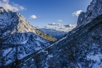
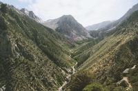
The following example shows three images of which two depict valleys in the mountains and one depicts fireworks. Therefore, the fireworks image is in comparison rather low in typicality in this set of images (i.e., atypical). It is important to note that an image’s typicality score highly depends on the reference set to which the image is compared to.
# Example images depicting valleys: valley_white, valley_green
# Example image depicting fireworks: fireworks
valley_white <- img_read(system.file('example_images', 'valley_white.jpg', package = 'imagefluency'))
valley_green <- img_read(system.file('example_images', 'valley_green.jpg', package = 'imagefluency'))
fireworks <- img_read(system.file('example_images', 'fireworks.jpg', package = 'imagefluency'))

# create image set as list
imglist <- list(valley_white, fireworks, valley_green)

# get typicality
img_typicality(imglist)
Calculating the typicality scores for the three images gives the following result:

Summary
imagefluency is an simple R package for
image fluency scores. The package allows to get scores for several basic
aesthetic principles that facilitate fluent cognitive processing of
images. It straightforward to use and allows for an easy conversion of
unstructured data into structured image features. These structured image
features are naturally interpretable (i.e., no black-box-model).
Finally, including such image information in statistical models might
increase a model’s statistical and predictive power.